Notes

What are the patient characteristics that predict worsening depression/anxiety in COPD patients?

Dataset of 101 Chronic obstructive pulmonary disease COPD patients.
The HAD variable is the score from the Hospital Anxiety and Depression scale.
HADS score ranges from 0 to 21

Choosing predictor variables

Characteristics: Age, Gender, PackHistory, Smoking.
Disease: CAT, COPDSEVERITY.
Lung function: FEV1, FEV1PRED, FVCPRED, FVCPRED1.
Co-morbidities:

Import Dataset

COPD <- read.csv("data/COPD_student_dataset.csv")

Missing or inaccurate values

Inspecting variables with summary() reveals some unlikely looking ranges.

summary(COPD[["HAD"]])

   Min. 1st Qu.  Median    Mean 3rd Qu.    Max. 
   0.00    6.00   10.00   11.18   15.00   56.20

The HAD score should range from 0 to 21, so there’s a least 1 incorrect value.

sum(COPD[["HAD"]] > 21)

[1] 11

table(COPD[["HAD"]][COPD[["HAD"]] > 21])


  22   23   26   29   30 56.2 
   3    2    2    1    2    1

In fact there are 11 values over 21. It looks as though the scale for this actually runs from 0 to 30. I’d like to take these questions back to the research team to confirm, but for the sake of this exercise I will just ignore 56.2 as the outlier.

COPD[["HAD"]][COPD[["HAD"]] > 30] <- NA_integer_

Similarly, CAT has a clearly separated max value. CAT is the COPD assessment test and according to the CAT user guide is scored on a scale of 0-40.

summary(COPD[["CAT"]])

   Min. 1st Qu.  Median    Mean 3rd Qu.    Max. 
   3.00   12.00   18.00   19.34   24.00  188.00

sum(COPD[["CAT"]] > 40)

[1] 1

Since there is just the one, I will exclude it.

COPD[["CAT"]][COPD[["CAT"]] > 40] <- NA_integer_

Collinearity of predictor candidates

Correlation in continuous variables

continuous_vars <- c("PackHistory", "CAT", "FEV1", 
                     "FEV1PRED", "FVC", "FVCPRED")

Pairwise scatterplots
Correlation Matrix

pairs(COPD[, continuous_vars])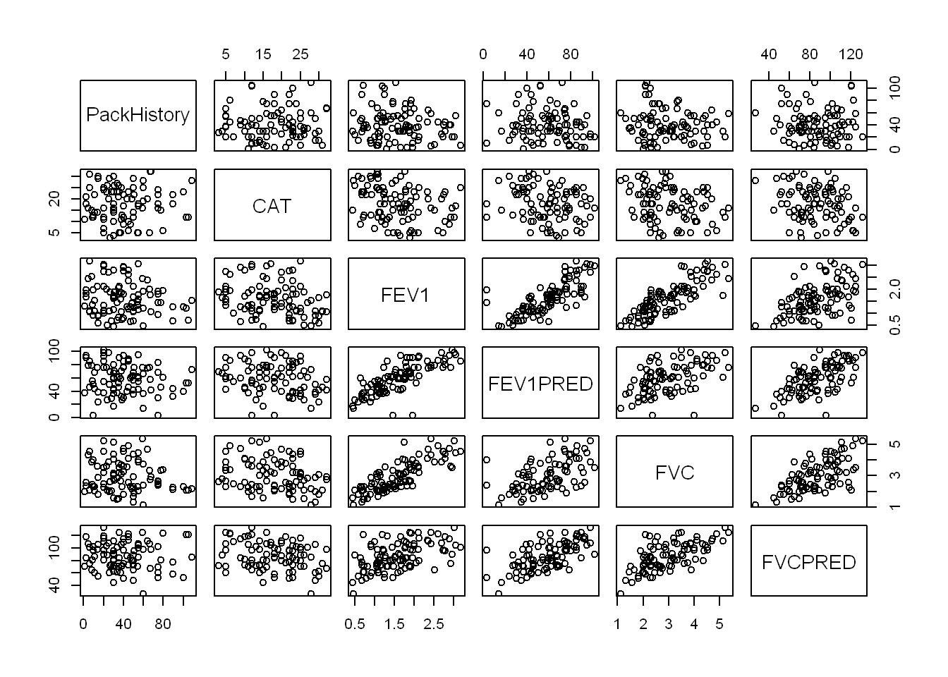

cor(COPD[, continuous_vars])

             PackHistory CAT       FEV1   FEV1PRED         FVC      FVCPRED
PackHistory  1.000000000  NA -0.1315051 -0.1313410 -0.09307289 -0.004489788
CAT                   NA   1         NA         NA          NA           NA
FEV1        -0.131505136  NA  1.0000000  0.7761105  0.82016501  0.515856013
FEV1PRED    -0.131340964  NA  0.7761105  1.0000000  0.52152997  0.625877533
FVC         -0.093072888  NA  0.8201650  0.5215300  1.00000000  0.622430376
FVCPRED     -0.004489788  NA  0.5158560  0.6258775  0.62243038  1.000000000

Lung Function

There is strong correlation between the lung function measures FEV1, FEV1PRED, FVC and FVCPRED, so I will seek to include only one of the four, by exploring the individual relationships of each to HAD:

FEV1_model <- lm(HAD ~ FEV1, COPD)
summary(FEV1_model)


Call:
lm(formula = HAD ~ FEV1, data = COPD)

Residuals:
    Min      1Q  Median      3Q     Max 
-11.869  -4.710  -1.278   3.932  18.128 

Coefficients:
            Estimate Std. Error t value Pr(>|t|)    
(Intercept)   14.622      1.858   7.871 4.78e-12 ***
FEV1          -2.435      1.072  -2.272   0.0253 *  
---
Signif. codes:  0 '***' 0.001 '**' 0.01 '*' 0.05 '.' 0.1 ' ' 1

Residual standard error: 7.188 on 98 degrees of freedom
  (1 observation deleted due to missingness)
Multiple R-squared:  0.05004,   Adjusted R-squared:  0.04035 
F-statistic: 5.162 on 1 and 98 DF,  p-value: 0.02527

plot(HAD ~ FEV1, COPD)
abline(FEV1_model)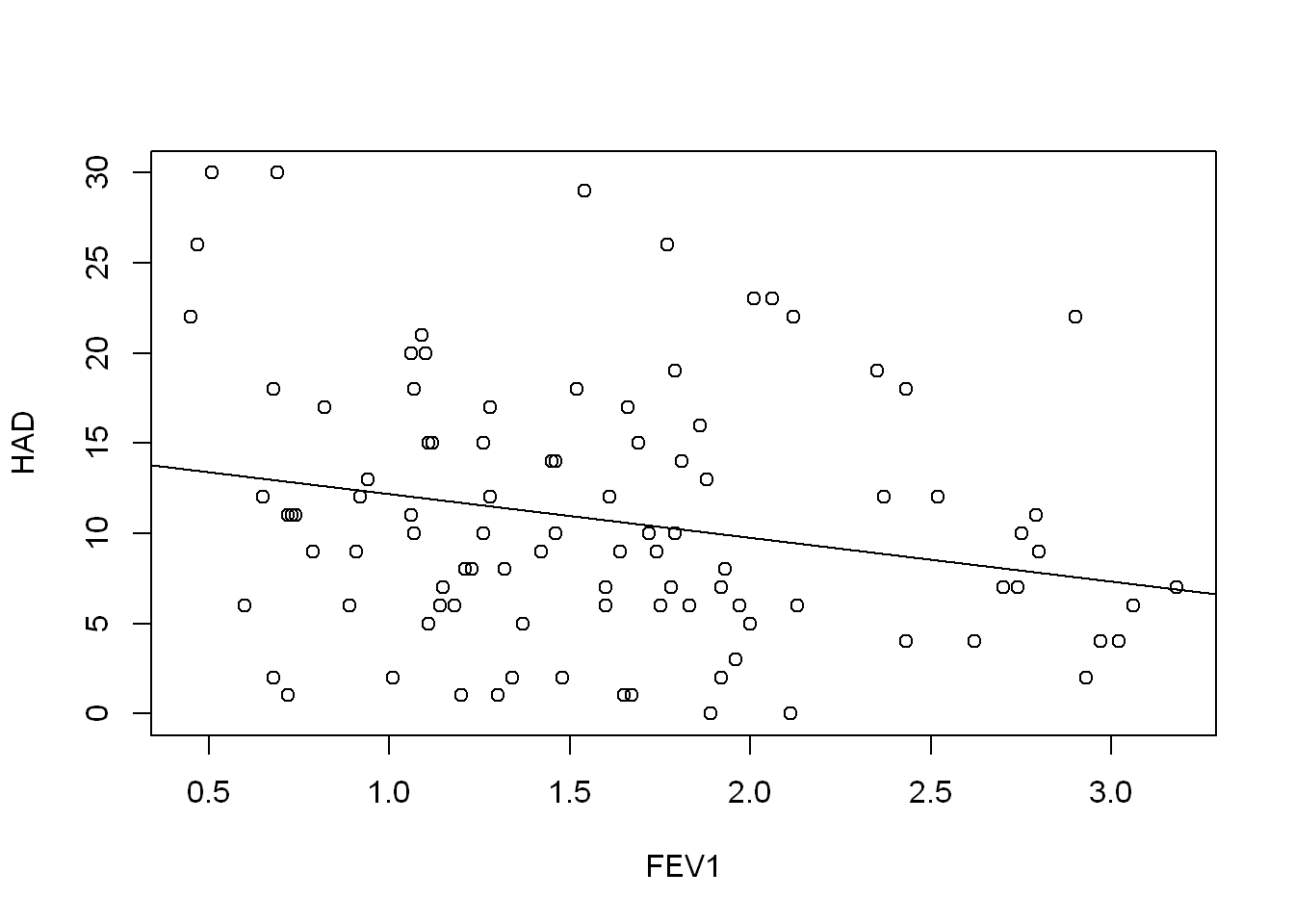

FEV1PRED_model <- lm(HAD ~ FEV1PRED, COPD)
summary(FEV1PRED_model)


Call:
lm(formula = HAD ~ FEV1PRED, data = COPD)

Residuals:
    Min      1Q  Median      3Q     Max 
-11.819  -4.662  -1.654   4.731  19.298 

Coefficients:
            Estimate Std. Error t value Pr(>|t|)    
(Intercept) 15.06450    2.02895   7.425 4.19e-11 ***
FEV1PRED    -0.07448    0.03260  -2.284   0.0245 *  
---
Signif. codes:  0 '***' 0.001 '**' 0.01 '*' 0.05 '.' 0.1 ' ' 1

Residual standard error: 7.186 on 98 degrees of freedom
  (1 observation deleted due to missingness)
Multiple R-squared:  0.05056,   Adjusted R-squared:  0.04087 
F-statistic: 5.218 on 1 and 98 DF,  p-value: 0.02451

plot(HAD ~ FEV1PRED, COPD)
abline(FEV1PRED_model)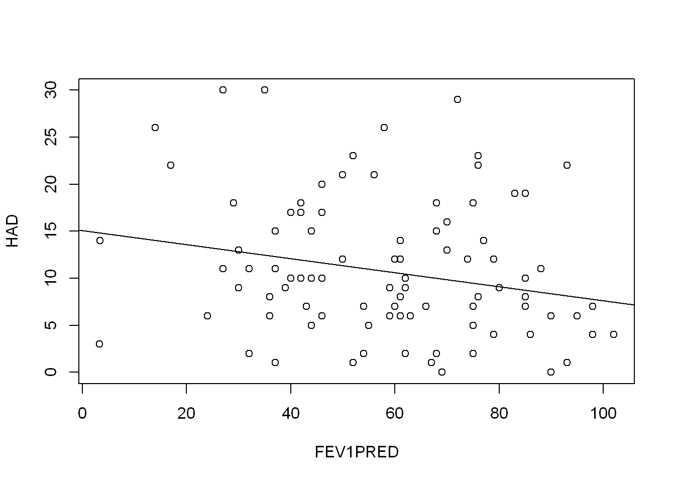

FVC_model <- lm(HAD ~ FVC, COPD)
summary(FVC_model)


Call:
lm(formula = HAD ~ FVC, data = COPD)

Residuals:
    Min      1Q  Median      3Q     Max 
-11.161  -5.108  -1.560   4.502  18.147 

Coefficients:
            Estimate Std. Error t value Pr(>|t|)    
(Intercept)  14.4460     2.3162   6.237 1.13e-08 ***
FVC          -1.2586     0.7448  -1.690   0.0943 .  
---
Signif. codes:  0 '***' 0.001 '**' 0.01 '*' 0.05 '.' 0.1 ' ' 1

Residual standard error: 7.269 on 98 degrees of freedom
  (1 observation deleted due to missingness)
Multiple R-squared:  0.02831,   Adjusted R-squared:  0.01839 
F-statistic: 2.855 on 1 and 98 DF,  p-value: 0.09426

plot(HAD ~ FVC, COPD)
abline(FVC_model)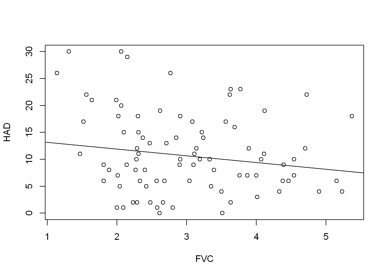

FVCPRED_model <- lm(HAD ~ FVCPRED, COPD)
summary(FVCPRED_model)


Call:
lm(formula = HAD ~ FVCPRED, data = COPD)

Residuals:
    Min      1Q  Median      3Q     Max 
-12.010  -5.014  -1.193   4.286  19.529 

Coefficients:
            Estimate Std. Error t value Pr(>|t|)    
(Intercept)  18.5253     2.9301   6.322 7.66e-09 ***
FVCPRED      -0.0905     0.0330  -2.742  0.00725 ** 
---
Signif. codes:  0 '***' 0.001 '**' 0.01 '*' 0.05 '.' 0.1 ' ' 1

Residual standard error: 7.107 on 98 degrees of freedom
  (1 observation deleted due to missingness)
Multiple R-squared:  0.07127,   Adjusted R-squared:  0.06179 
F-statistic:  7.52 on 1 and 98 DF,  p-value: 0.007254

plot(HAD ~ FVCPRED, COPD)
abline(FVCPRED_model)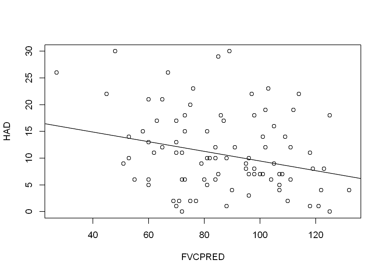

They all have seem to be a slight negative predictor of HAD, but none of them explain the variation very well. The FVCPRED model has the highest adjusted R squared value at 0.06179.

PackHistory and smoking

PackHistory and smoking are both about a person’s smoking history. smoking is a categorical variable with value 1 for has smoked previously and 2 for currently smokes. PackHistory records a person’s pack years smoking, where pack years is defined as twenty cigarettes smoked every day for one year.

table(COPD[["smoking"]])


 1  2 
16 85

cor(COPD[["smoking"]], COPD[["PackHistory"]], method = "spearman")

[1] -0.02234481

They don’t appear to be highly correlated, but I still don’t think I want to include both. “smoking” is probably not that helpful given there are such a small number aren’t current smokers. I still want a bit more of a comparison though.

boxplot(COPD[["smoking"]], COPD[["PackHistory"]],
        xlab = "Smoking status",
        ylab = "Years of daily pack smoking")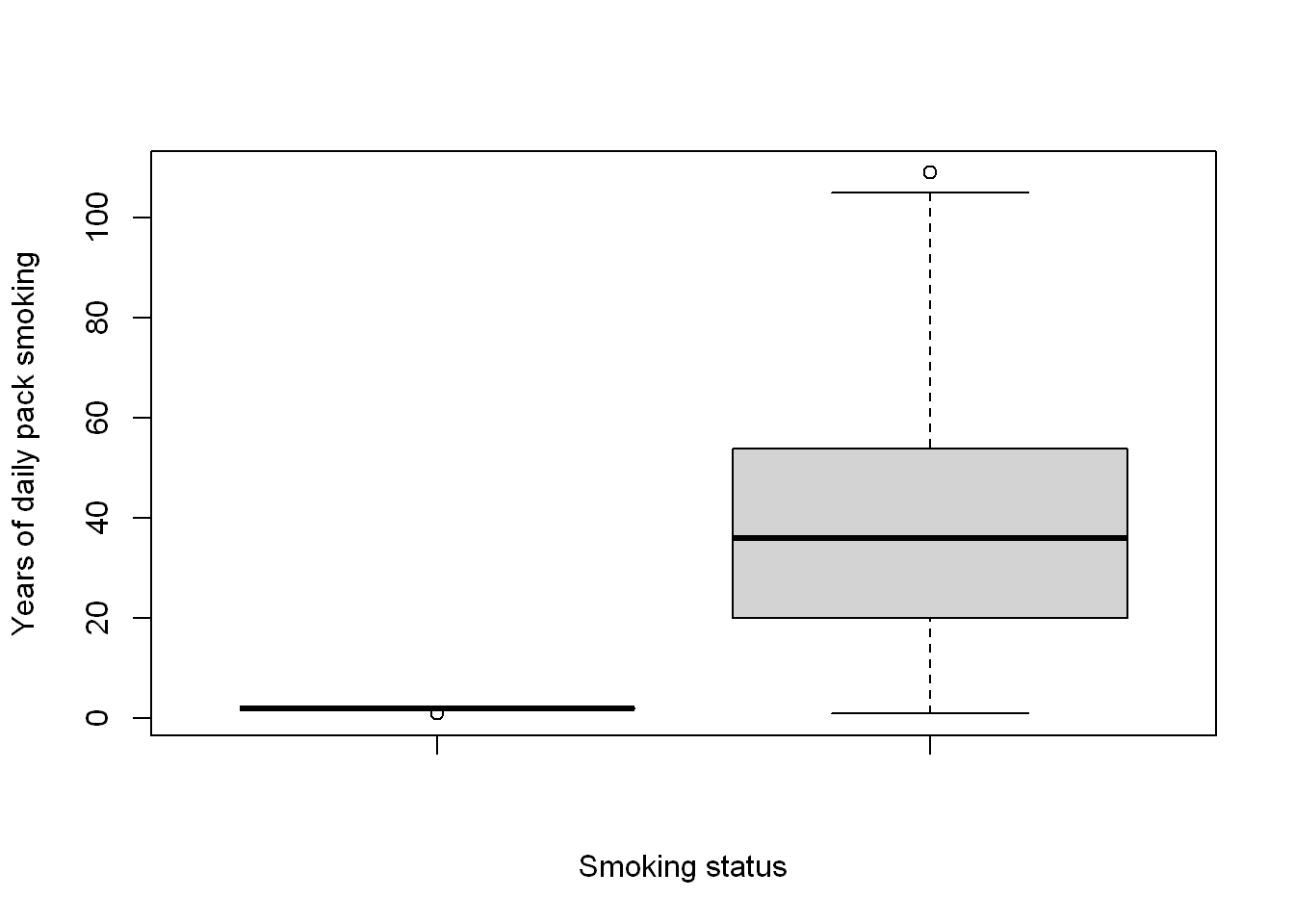

Well, this has raised some concerns to me about PackHistory. If the unit is years the the number with 80+ looks suprising.

sum(COPD[["PackHistory"]] > 80)

[1] 6

Ok, it’s only 6 which is not too bad, but since there is an AGE column I want to check how possible this is.

sum(COPD[["PackHistory"]] > COPD[["AGE"]])

[1] 14

This feels a bit problematic. I’m not sure if the description I have about the measure is incorrect, or if it’s the data, but as this is >10% of the dataset that looks impossible I think I’m going to have to ignore the this as a potential predictor. That’s also without adjusting for some assumption of a reasonable age people might start smoking.

Comorbidities

There are several binary variables relating to comorbidity

COPD$comorbid <- COPD$Diabetes == 1 | COPD$muscular == 1 | 
  COPD$hypertension == 1 | COPD$AtrialFib == 1 | COPD$IHD == 1

COPD$comorbid <- factor(COPD$comorbid)

Disease measure

CAT and COPDSEVERITY are both measures of COPD disease status. CAT is a continuous score and COPDSEVERITY has three categories of severity. If both variables are suitable I will select the more detailed CAT.

CAT
COPDSEVERITY

summary(COPD[["CAT"]])

   Min. 1st Qu.  Median    Mean 3rd Qu.    Max.    NA's 
   3.00   12.00   18.00   17.65   23.25   32.00       1

summary(lm(HAD ~ CAT, COPD))


Call:
lm(formula = HAD ~ CAT, data = COPD)

Residuals:
     Min       1Q   Median       3Q      Max 
-11.5470  -4.1719  -0.9636   3.5531  15.6532 

Coefficients:
            Estimate Std. Error t value Pr(>|t|)    
(Intercept)  1.69666    1.51963   1.116    0.267    
CAT          0.51668    0.07896   6.544 2.84e-09 ***
---
Signif. codes:  0 '***' 0.001 '**' 0.01 '*' 0.05 '.' 0.1 ' ' 1

Residual standard error: 6.161 on 97 degrees of freedom
  (2 observations deleted due to missingness)
Multiple R-squared:  0.3063,    Adjusted R-squared:  0.2991 
F-statistic: 42.82 on 1 and 97 DF,  p-value: 2.839e-09

table(COPD[["COPDSEVERITY"]])


       MILD    MODERATE      SEVERE VERY SEVERE 
         23          43          27           8

summary(lm(HAD ~ COPDSEVERITY, COPD))


Call:
lm(formula = HAD ~ COPDSEVERITY, data = COPD)

Residuals:
    Min      1Q  Median      3Q     Max 
-11.148  -5.116  -1.148   3.884  18.884 

Coefficients:
                        Estimate Std. Error t value Pr(>|t|)    
(Intercept)                8.273      1.524   5.429 4.26e-07 ***
COPDSEVERITYMODERATE       1.844      1.874   0.984   0.3276    
COPDSEVERITYSEVERE         3.875      2.053   1.888   0.0621 .  
COPDSEVERITYVERY SEVERE    7.727      2.951   2.619   0.0103 *  
---
Signif. codes:  0 '***' 0.001 '**' 0.01 '*' 0.05 '.' 0.1 ' ' 1

Residual standard error: 7.147 on 96 degrees of freedom
  (1 observation deleted due to missingness)
Multiple R-squared:  0.07984,   Adjusted R-squared:  0.05108 
F-statistic: 2.777 on 3 and 96 DF,  p-value: 0.04542

Trying out the variables as predictors

That leaves us with the following candidate predictor variables to explore

AGE
gender
CAT
FVCPRED
comorbid

It is known that age and gender impact depression. One might expect people with a worse disease condition i.e. higher CAT score to also have a worse HAD score. First I want to explore the relationship of each variable individually with the outcome HAD.

Characteristics

age_lm <- lm(HAD ~ AGE, COPD)
summary(age_lm)


Call:
lm(formula = HAD ~ AGE, data = COPD)

Residuals:
    Min      1Q  Median      3Q     Max 
-12.554  -4.407  -1.103   3.659  20.081 

Coefficients:
            Estimate Std. Error t value Pr(>|t|)    
(Intercept) 25.50974    6.43149   3.966 0.000139 ***
AGE         -0.21069    0.09111  -2.312 0.022843 *  
---
Signif. codes:  0 '***' 0.001 '**' 0.01 '*' 0.05 '.' 0.1 ' ' 1

Residual standard error: 7.181 on 98 degrees of freedom
  (1 observation deleted due to missingness)
Multiple R-squared:  0.05174,   Adjusted R-squared:  0.04207 
F-statistic: 5.348 on 1 and 98 DF,  p-value: 0.02284

confint(age_lm)

                 2.5 %      97.5 %
(Intercept) 12.7466586 38.27282554
AGE         -0.3914899 -0.02988553

The model suggests that for every 1 year of age, HAD score decreases by 0.21. So there does appear to be some relationship, but it doesn’t explain the variation in HAD very well.

plot(HAD ~ AGE, COPD)
abline(age_lm)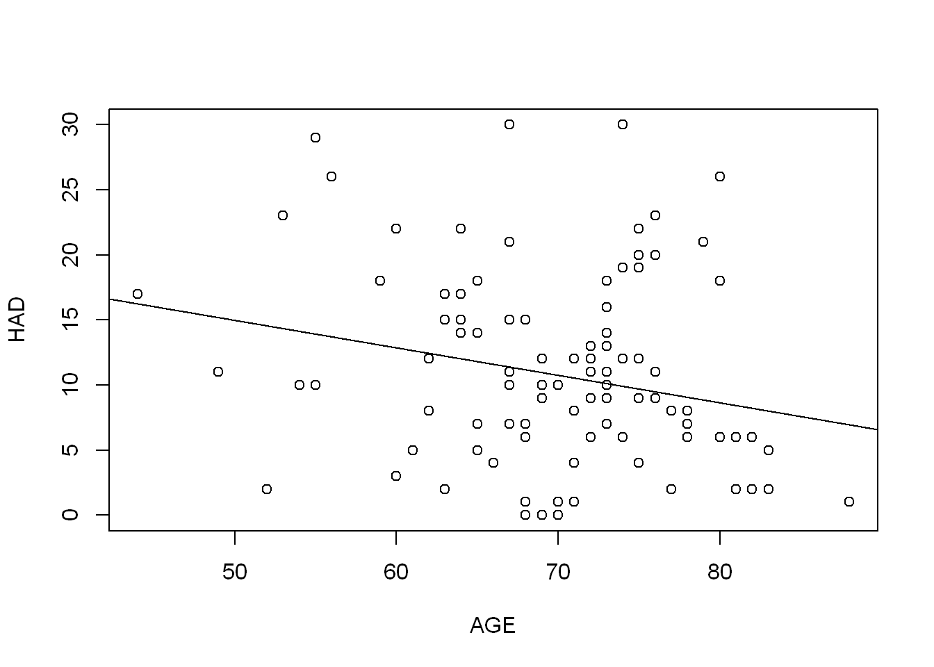

gender_lm <- lm(HAD ~ gender, COPD)
summary(gender_lm)


Call:
lm(formula = HAD ~ gender, data = COPD)

Residuals:
    Min      1Q  Median      3Q     Max 
-12.000  -4.046  -1.023   4.954  18.000 

Coefficients:
            Estimate Std. Error t value Pr(>|t|)    
(Intercept)   12.000      1.236   9.706 5.26e-16 ***
gender        -1.954      1.533  -1.274    0.206    
---
Signif. codes:  0 '***' 0.001 '**' 0.01 '*' 0.05 '.' 0.1 ' ' 1

Residual standard error: 7.314 on 98 degrees of freedom
  (1 observation deleted due to missingness)
Multiple R-squared:  0.0163,    Adjusted R-squared:  0.006257 
F-statistic: 1.623 on 1 and 98 DF,  p-value: 0.2056

confint(gender_lm)

                2.5 %    97.5 %
(Intercept)  9.546528 14.453472
gender      -4.997004  1.089311

The p-value of 0.2 means we cannot rule out the null hypothesis of gender having no relationship to HAD score, and indeed the 95% confidence interval includes a gradient of 0. I will continue to explore this with gender alongside other variables.

boxplot(HAD ~ gender, COPD)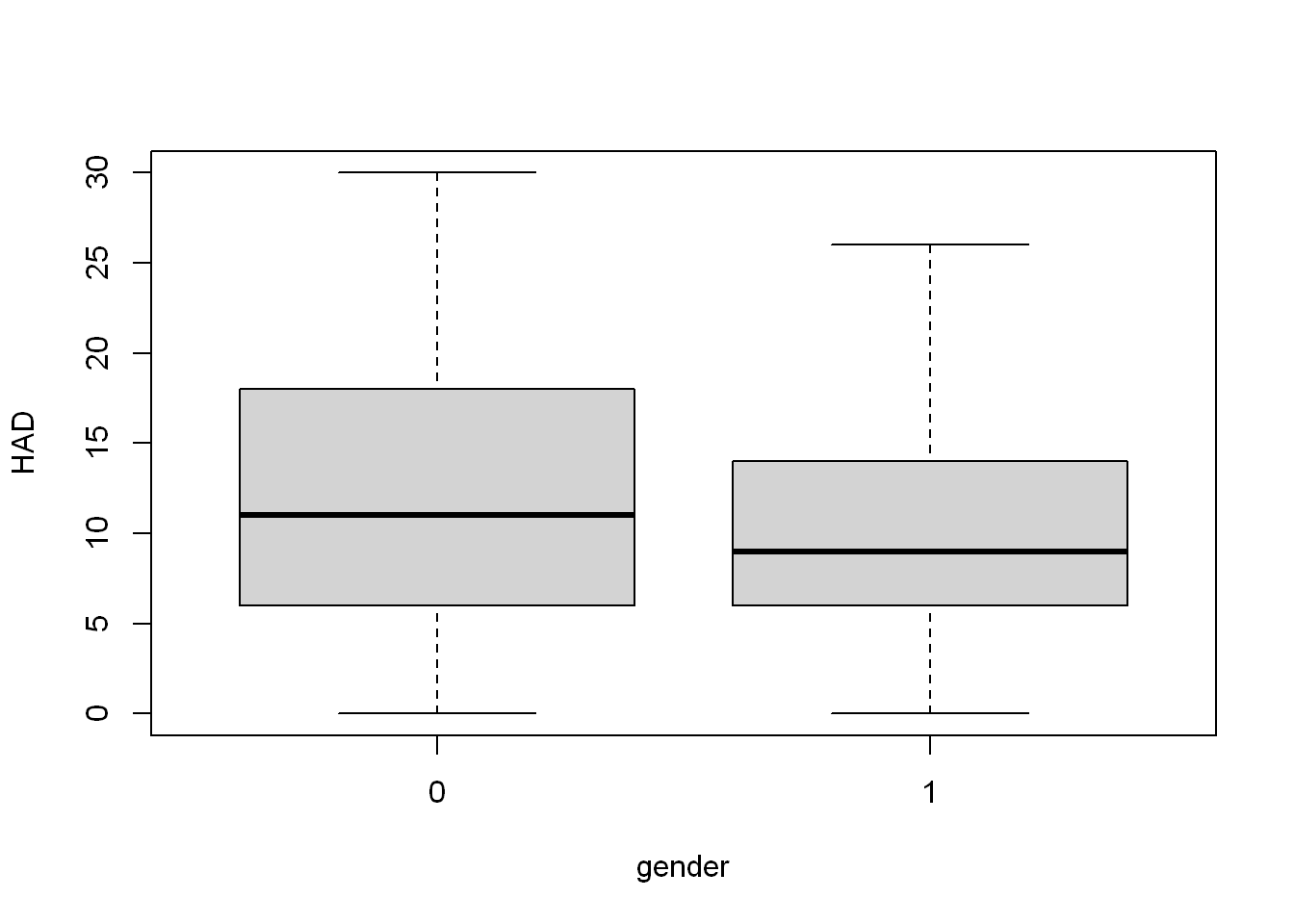

We can see the HAD score distribution is fairly similar in men and women. I do want to check out age and gender alongside each other.

age_gender_lm <- lm(HAD ~ AGE + gender, COPD)
summary(age_gender_lm)


Call:
lm(formula = HAD ~ AGE + gender, data = COPD)

Residuals:
     Min       1Q   Median       3Q      Max 
-11.8001  -4.6953  -0.8481   4.1130  19.0821 

Coefficients:
            Estimate Std. Error t value Pr(>|t|)    
(Intercept) 25.51495    6.43430   3.965  0.00014 ***
AGE         -0.19726    0.09222  -2.139  0.03496 *  
gender      -1.45745    1.52404  -0.956  0.34129    
---
Signif. codes:  0 '***' 0.001 '**' 0.01 '*' 0.05 '.' 0.1 ' ' 1

Residual standard error: 7.184 on 97 degrees of freedom
  (1 observation deleted due to missingness)
Multiple R-squared:  0.0606,    Adjusted R-squared:  0.04123 
F-statistic: 3.129 on 2 and 97 DF,  p-value: 0.04822

Do they have an impact through intersection?

age_gender_lm <- lm(HAD ~ AGE * gender, COPD)
summary(age_gender_lm)


Call:
lm(formula = HAD ~ AGE * gender, data = COPD)

Residuals:
     Min       1Q   Median       3Q      Max 
-13.2680  -4.4037  -0.9083   3.9165  18.4149 

Coefficients:
            Estimate Std. Error t value Pr(>|t|)
(Intercept)  9.59955   12.64044   0.759    0.449
AGE          0.03504    0.18365   0.191    0.849
gender      19.93655   14.73321   1.353    0.179
AGE:gender  -0.30942    0.21196  -1.460    0.148

Residual standard error: 7.143 on 96 degrees of freedom
  (1 observation deleted due to missingness)
Multiple R-squared:  0.081, Adjusted R-squared:  0.05228 
F-statistic: 2.821 on 3 and 96 DF,  p-value: 0.04299

It doesn’t appear to be the case and seems like it might be more valuable to include AGE without gender.

Disease

cat_lm <- lm(HAD ~ CAT, COPD)
summary(cat_lm)


Call:
lm(formula = HAD ~ CAT, data = COPD)

Residuals:
     Min       1Q   Median       3Q      Max 
-11.5470  -4.1719  -0.9636   3.5531  15.6532 

Coefficients:
            Estimate Std. Error t value Pr(>|t|)    
(Intercept)  1.69666    1.51963   1.116    0.267    
CAT          0.51668    0.07896   6.544 2.84e-09 ***
---
Signif. codes:  0 '***' 0.001 '**' 0.01 '*' 0.05 '.' 0.1 ' ' 1

Residual standard error: 6.161 on 97 degrees of freedom
  (2 observations deleted due to missingness)
Multiple R-squared:  0.3063,    Adjusted R-squared:  0.2991 
F-statistic: 42.82 on 1 and 97 DF,  p-value: 2.839e-09

confint(cat_lm)

                 2.5 %    97.5 %
(Intercept) -1.3193823 4.7127094
CAT          0.3599729 0.6733953

As a measure of disease I would expect CAT score to predict increased HAD score. Indeed, CAT looks like it’s going to be valuable to include, there is a clear positive relationship with HAD. That there is no relationship can be ruled out even at significance levels below 0.001.

plot(HAD ~ CAT, COPD)
abline(cat_lm, col = "blue")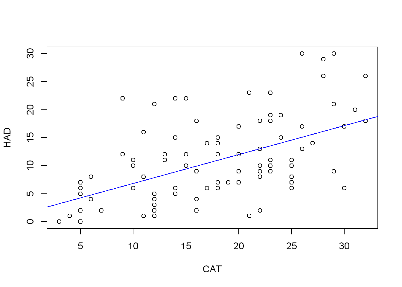

Comorbidities

comorbid_lm <- lm(HAD ~ comorbid, COPD)
summary(comorbid_lm)


Call:
lm(formula = HAD ~ comorbid, data = COPD)

Residuals:
     Min       1Q   Median       3Q      Max 
-10.7593  -5.5811  -0.7593   4.6689  20.4783 

Coefficients:
             Estimate Std. Error t value Pr(>|t|)    
(Intercept)     9.522      1.075   8.861 3.58e-14 ***
comorbidTRUE    2.238      1.462   1.530    0.129    
---
Signif. codes:  0 '***' 0.001 '**' 0.01 '*' 0.05 '.' 0.1 ' ' 1

Residual standard error: 7.288 on 98 degrees of freedom
  (1 observation deleted due to missingness)
Multiple R-squared:  0.02333,   Adjusted R-squared:  0.01337 
F-statistic: 2.341 on 1 and 98 DF,  p-value: 0.1292

confint(comorbid_lm)

                  2.5 %    97.5 %
(Intercept)   7.3892986 11.654180
comorbidTRUE -0.6643639  5.139404

No clear indication, but I want to check out if comorbodity interacts with disease/condition.

cat_comorbid_lm <- lm(HAD ~ CAT + comorbid + CAT * comorbid, COPD)
summary(cat_comorbid_lm)


Call:
lm(formula = HAD ~ CAT + comorbid + CAT * comorbid, data = COPD)

Residuals:
    Min      1Q  Median      3Q     Max 
-11.662  -3.998  -1.844   4.023  15.492 

Coefficients:
                 Estimate Std. Error t value Pr(>|t|)    
(Intercept)        0.2758     2.0973   0.132    0.896    
CAT                0.5474     0.1119   4.890 4.09e-06 ***
comorbidTRUE       3.0817     3.0425   1.013    0.314    
CAT:comorbidTRUE  -0.0790     0.1584  -0.499    0.619    
---
Signif. codes:  0 '***' 0.001 '**' 0.01 '*' 0.05 '.' 0.1 ' ' 1

Residual standard error: 6.158 on 95 degrees of freedom
  (2 observations deleted due to missingness)
Multiple R-squared:  0.3213,    Adjusted R-squared:  0.2999 
F-statistic: 14.99 on 3 and 95 DF,  p-value: 4.586e-08

The relationship looks weaker, but I will note that the adjusted R squared is slightly higher than that of \(CAT\) on it’s own, so it may better explain the variance, but p-values for both \(comorbid\) and \(CAT * comorbid\) are very high, making their null hypotheses significantly likely.

Selecting multiple variabels

more multiple combinations to make my final variable selection.I’m confident I want to include CAT, but want to try out some

multi_lm1 <- lm(HAD ~ CAT + FVCPRED + AGE + gender + comorbid, COPD)
summary(multi_lm1)


Call:
lm(formula = HAD ~ CAT + FVCPRED + AGE + gender + comorbid, data = COPD)

Residuals:
     Min       1Q   Median       3Q      Max 
-10.0897  -4.2262  -0.7329   2.7345  16.7165 

Coefficients:
             Estimate Std. Error t value Pr(>|t|)    
(Intercept)  17.90909    6.42997   2.785  0.00648 ** 
CAT           0.45935    0.08132   5.648 1.75e-07 ***
FVCPRED      -0.03636    0.03000  -1.212  0.22849    
AGE          -0.17148    0.07770  -2.207  0.02977 *  
gender       -1.72259    1.29278  -1.332  0.18596    
comorbidTRUE  1.96907    1.22192   1.611  0.11047    
---
Signif. codes:  0 '***' 0.001 '**' 0.01 '*' 0.05 '.' 0.1 ' ' 1

Residual standard error: 5.962 on 93 degrees of freedom
  (2 observations deleted due to missingness)
Multiple R-squared:  0.3772,    Adjusted R-squared:  0.3437 
F-statistic: 11.26 on 5 and 93 DF,  p-value: 1.658e-08

confint(multi_lm1)

                   2.5 %      97.5 %
(Intercept)   5.14043738 30.67774911
CAT           0.29785634  0.62084225
FVCPRED      -0.09592529  0.02320335
AGE          -0.32577467 -0.01718824
gender       -4.28980514  0.84461913
comorbidTRUE -0.45740822  4.39555591

This does bring the adjusted R-squared higher, but as with CAT and comorbid, FVCPRED, comorbid and gender have high p-values.

I’m not sure how best to interpret all of that together, but it does make me think it may be best to try just CAT and AGE.

cat_age_lm <- lm(HAD ~ CAT + AGE, COPD)
summary(cat_age_lm)


Call:
lm(formula = HAD ~ CAT + AGE, data = COPD)

Residuals:
     Min       1Q   Median       3Q      Max 
-11.3435  -4.1107  -0.5489   3.4906  16.4015 

Coefficients:
            Estimate Std. Error t value Pr(>|t|)    
(Intercept) 13.93262    5.71519   2.438   0.0166 *  
CAT          0.50484    0.07759   6.506 3.49e-09 ***
AGE         -0.17170    0.07743  -2.218   0.0289 *  
---
Signif. codes:  0 '***' 0.001 '**' 0.01 '*' 0.05 '.' 0.1 ' ' 1

Residual standard error: 6.04 on 96 degrees of freedom
  (2 observations deleted due to missingness)
Multiple R-squared:  0.3401,    Adjusted R-squared:  0.3263 
F-statistic: 24.73 on 2 and 96 DF,  p-value: 2.169e-09

confint(cat_age_lm)

                 2.5 %      97.5 %
(Intercept)  2.5880619 25.27718425
CAT          0.3508179  0.65886693
AGE         -0.3253919 -0.01801275

My feeling is this is the best model of the ones I’ve tried. Both CAT and AGE seem to have explanatory power over their respective null hypotheses. The adjusted R-squared value is higher than most of the other models I’ve tried at \(0.33\), but that’s still quite low if the potential max is 1, and so suggests not giving a great explanation of the variation.

I feel like I’m missing something, but I think this is my best first shot:

\(HAD = 13.93 + 0.50 * CAT - 0.17 * AGE\)